This entry focuses around the concept of a height map and in the process will introduce many other important concepts. The first thing we want to implement in this process is a new grid object where we can control both the size and the number of rows and columns in the grid. This creates a very versatile control that can be used to render a single square all the way up to an extremely granular grid. The reason this is important is because many interactions we perform are done on a per-vertex basis, therefore by increasing the number of vertices we can introduce more detailed effects.

Using the same pattern I used to construct the cube in previous examples I will create a new Grid class: class Grid(gl: GL4, xwidth: Float, xcount: Int, zwidth: Float, zcount: Int) extends Matrices with Movable with Rotatable

The initialization of the grid is pretty straight forward: val maxWidth = xwidth * xcount; val maxLen = zwidth * zcount * -1; for(x <- 0 until xcount) { for(z <- 0 until zcount) { val xpos: Float = x * xwidth; val zpos: Float = z * zwidth * -1; //Negative -1 to render it down the z-axis addVertex(xpos, 0.0f, zpos); addTexture(xpos / maxWidth, zpos / maxLen, 0.0f); addVertex(xpos + xwidth, 0.0f, zpos - zwidth); addTexture((xpos + xwidth) / maxWidth, (zpos - zwidth) / maxLen, 0.0f); addVertex(xpos, 0.0f, zpos - zwidth); addTexture(xpos / maxWidth, (zpos - zwidth) / maxLen, 0.0f); addVertex(xpos, 0.0f, zpos); addTexture(xpos / maxWidth, zpos / maxLen, 0.0f); addVertex(xpos + xwidth, 0.0f, zpos); addTexture((xpos + xwidth) / maxWidth, zpos / maxLen, 0.0f); addVertex(xpos + xwidth, 0.0f, zpos - zwidth); addTexture((xpos + xwidth) / maxWidth, (zpos - zwidth) / maxLen, 0.0f); } }

It is important to not lose track of the orientation of the z-axis. We are going to start the grid at position (0,0) on the xz axis and work our way down the positive x axis and the negative z axis. For this case I am going to only generate vertices and texture coordinates for the grid, the color and normals will be added in at other stages. Texture coordinates are respresented by a two-value pair with numbers that range from 0.0 to 1.0 to represent the coordinates of our 2D picture. We calculate these coordinates by dividing our vertex coordinates by the maximum values to convert them to a number between 0.0 and 1.0.

In order to render the height map we will need to introduce a new shader that can properly handle this texture data and convert it into vertical coordinates. This step will need to be performed at the beginning of our pipeline in the vertex shader before we attempt to do anything else with that vertex: void main(void) { //Fetch the color value of the texture at the given coordinates vec4 texColor = texture(s, texCoords.xy); //Re-calculate the vertex position by increasing the y-location based on the color of the texture //The texture is greyscale so all three components in the vector should be the same. We do however want //to multiplay the value by a scaling amount to increase the height of the terrain vec4 newPosition = vec4(position.x, position.y + texColor.y * 5.0, position.z, position.w); gl_Position = pMatrix * mvMatrix * newPosition; //mvPosition will contain the vector position modified by the mvMatrix, we need this because the position the //geometry shader normally gets will also be modified by the projection matrix and therefore be unsuitable //for lighting calculations mvPosition = vec3(mvMatrix * newPosition); lightPos = vec3(0.0, 1.0, 1.0); //This will just pass through the color to the geometry shader where the intensity will be actually calculated intensity = color; }

The first line here samples the texture color at the texture coordinates that were fed into the shader. The four component vector returned represents the texture color, but since we know it is greyscale then we know we can pull the value out of any of the first three components and achieve the same effect. The value we pull out of that vector will be a value between 0 (black) and 1 (white) representing the height of the terrain at that location. Using that value we create our new position using the original position fed into the shader and modifying the y-position with our new value.

Unfortunately, now that we have changed the y-position of that vertex we can no longer use any pre-calculated normal vector for the grid since the resulting triangle is now facing a new direction. Somehow we need to calculate a new normal vector based on the new vertex coordinates in order for us to properly calculate the lighting for the height map.

A well known way to compute a new normal vector for a triangle is by performing a cross product of two of the vectors that make up the triangle. Unfortunately we do not have the information we need to perform the cross product in the vertex shader since it is only capable of computing a single vertex at a time. To calculate our cross product we need to introduce a new shader into the pipeline called a geometry shader. This shader will execute inbetween the vertex and fragment shaders and allows us to see all three vertices that make up our triangle at once.

Using this information we can calculate the two vectors that make up the triangle and then perform the cross product on them to find our new normal vector. in vec3 mvPosition[]; in vec3 lightPos[]; in vec4 intensity[]; out vec4 gIntensity; void main(void) { int i; //Calculate the normal for the triangle, this will be the same for all vertices vec4 ab = normalize(gl_in[0].gl_Position - gl_in[1].gl_Position); vec4 bc = normalize(gl_in[1].gl_Position - gl_in[2].gl_Position); //The cross product of two vectors will create a new vector that points in the direction //the plane created by the first two vectors is facing. In other words a normal vector. vec3 normal = normalize(cross(vec3(bc), vec3(ab))); //I wish I could explain this better. It appears that vertical surfaces generate a normal pointing //in the wrong direction. Reflecting it across the xy-plane fixes this problem normal.z = -normal.z; for(i = 0; i < gl_in.length(); i++) { gl_Position = gl_in[i].gl_Position; //Calculate the intensity based off the light position and calculated normal vec3 vLight = normalize(lightPos[i] - mvPosition[i]); gIntensity = (max(dot(vLight, normal), 0.0) + 0.0) * intensity[i]; EmitVertex(); } EndPrimitive(); }

You can see at the top here that our inputs are slightly different. They share the same names as the outputs from our vertex shader but they are now arrays of values rather than single values. This works well for us because now that we have all three vertices of our triangle we can compute the normal for it. Unfortunately the resulting normal is pointing the wrong way down the z-axis (I suspect this has something to do with how OpenGL orients the z-axis), but this can be easily fixed by negating the z-value and reflecting it across the plane formed by the xy-axis.

Once we have our normal we can finally compute the intensity of the color for all vertices in the triangle. This is easily done using the dot product calculation used in the previous blog entry.

With our shaders ready we can get ready to render our height map. The first step is to create our new shader program that consumes our new shader as well as all of our uniform and texture data. class HeightMapProgram(gl: GL4) extends GLProgram { init(); private def init(): Unit = { targetGL = gl; val createVertexShader = ShaderLoader.createShader(gl, GL2ES2.GL_VERTEX_SHADER, this.getClass())_; val createFragmentShader = ShaderLoader.createShader(gl, GL2ES2.GL_FRAGMENT_SHADER, this.getClass())_; val createGeometryShader = ShaderLoader.createShader(gl, GL3.GL_GEOMETRY_SHADER, this.getClass())_; val vShader: ShaderCode = createVertexShader("shaders/heightvshader.glsl"); if(vShader.compile(gl, System.out) == false) throw new Exception("Failed to compile vertex shader"); val fShader: ShaderCode = createFragmentShader("shaders/heightfshader.glsl"); if(fShader.compile(gl, System.out) == false) throw new Exception("Failed to compile fragment shader"); val gShader: ShaderCode = createGeometryShader("shaders/heightgshader.glsl"); if(gShader.compile(gl, System.out) == false) throw new Exception("Failed to compile geometry shader"); program = ShaderLoader.createProgram(gl, vShader, gShader, fShader); if(program.link(gl, System.out) == false) throw new Exception("Failed to link program"); //No longer needed vShader.destroy(gl); fShader.destroy(gl); } override def getVerticesIndex() = 0; override def getTexturesIndex() = 1; override def getNormalsIndex() = -1; override def getColorsIndex() = 2; override def getModelViewIndex() = 3; override def getITModelViewIndex() = 4; override def getProjectionIndex() = 5; }

The major differences here are the locations of the inputs and the fact that we are added a new shader to our pipeline when we create our program.

The next step is to initialize our grid and texture data in the main application's initialization. heightProgram = new HeightMapProgram(gl); grid = new Grid(gl, 0.1f, 200, 0.1f, 200); mapTexture = TextureIO.newTexture(this.getClass().getResourceAsStream("resources/heightmap2.jpg"), false, TextureIO.JPG);

The map texture is a simple greyscale image, you can find many good examples by searching for 'height map' on google images. You can also easily construct one yourself with a drawing application. Fundamentally a height map is very similar to a file generated by a 3D modeling application which makes it a great entry point into understanding how 3D modeling works because it is very easy to visualize how it all fits together.

The next step is to prepare our logic for actually rendering the height map: heightProgram.activate(); grid.reset(); grid.move(-10.0f, 0.0f, 10.0f); grid.rotateY(degrees); grid.move(0.0f, -5.0f, -15.0f); gl.glUniformMatrix4fv(heightProgram.getProjectionIndex(), 1, false, mvp.glGetMatrixf()); gl.glUniform4f(heightProgram.getColorsIndex(), 0.0f, 1.0f, 1.0f, 1.0f); mapTexture.bind(gl); grid.draw(heightProgram); heightProgram.deactivate();

To simplify the application I've chosen to insert the color data through a uniform variable. The interesting thing here is you can see how the map texture is bound to the program which we will then access in the shader through the 'sampler2D' uniform.

At this point you could run the application and render the height map. However you may notice something doesn't look quite light. This is because in some height maps you introduce the chance that two triangles facing the camera are located on overlapping x and y coordinates down the z axis. The application will attempt to render both at the same time which will play games with how things look.

To prevent this we need to enable a depth test which will ensure that only the front-most triangle will be rendered to the screen. Thankfully this step is reasonably easy. First we need to allocate bits for the depth test early in application initialization: val config: GLCapabilities = new GLCapabilities(GLProfile.getDefault()); config.setDepthBits(8);

Then we need to enable our depth test: override def init(drawable: GLAutoDrawable): Unit = { val gl: GL4 = drawable.getGL().getGL4(); //Enable culling, by default only triangles with vertices ordered in a counter clockwise order will be rendered gl.glEnable(GL.GL_CULL_FACE); gl.glEnable(GL.GL_DEPTH_TEST);

Finally we need to make sure to clear the depth bit at the start of each render, much like how we would clear the color of the screen: gl.glClear(GL.GL_DEPTH_BUFFER_BIT);

With all of this in place you can now run the application and render the height map based on the input picture you provided

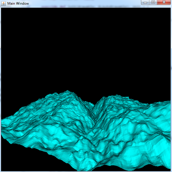
This is also a good way to demonstrate a common mechanism you see in graphics applications. By simple increasing or decreasing the number of rows and columns in the grid you can change how detailed the height map appears (at the cost of performance). You have likely seen a similar mechanism in modern games where lowering the graphic settings has caused characters to appear more blocky.

The goal of this entry will be to refine the previous implementation and focus more on the Scala aspects of the project since the previous article focused mostly on the OpenGL API. What we hope to achieve is the beginnings of a graphics API that we can reuse going forward to construct even more complex applications.

In the previous article I introduced a simple fixed point light shader program. My first goal is to encapsulate that program into a reusable class that will make it easier to use to render objects in future projects. However, I also want to design it in a way that it can be interchanged with other programs to achieve different effects. So the first thing I need to do is to create a base class that all of my future shader classes will inherit from. This base class will define what I expect to be common across future shader programs, specifically: initialization, destruction and locations of shader inputs. trait GLProgram { var program: ShaderProgram = null; var targetGL: GL4 = null; def getVerticesIndex(): Int; def getNormalsIndex(): Int; def getColorsIndex(): Int; def getModelViewIndex(): Int; def getITModelViewIndex(): Int; def getProjectionIndex(): Int; def activate(): Unit = { if(program == null || targetGL == null) return; program.useProgram(targetGL, true) } def destroy(): Unit = { if(program == null || targetGL == null) return; program.destroy(targetGL); } }

In this case I use a Scala trait to design my base class and it serves similar functionality to an abstract class in Java. The biggest difference between Scala traits and Java interfaces or abstract classes is not only can they contain implementation logic like an abstract class but you can mix multiple traits into a class much like interfaces (using the 'with' keyword), unlike Java applications which would only allow you to inherit from a single concrete class.

The trait above defines my activate method which will be called before I want to render something with the program, the destroy method to cleanup the program when it is no longer in use and a variety of get methods to obtain the indexes of the shader inputs. When my fixed point light shader class is implemented using this trait it looks like this: class FixedLightProgram(gl: GL4) extends GLProgram { init(); private def init(): Unit = { targetGL = gl; val createVertexShader = ShaderLoader.createShader(gl, GL2ES2.GL_VERTEX_SHADER, this.getClass())_; val createFragmentShader = ShaderLoader.createShader(gl, GL2ES2.GL_FRAGMENT_SHADER, this.getClass())_; val vShader: ShaderCode = createVertexShader("shaders/vshader.glsl"); if(vShader.compile(gl, System.out) == false) throw new Exception("Failed to compile vertex shader"); val fShader: ShaderCode = createFragmentShader("shaders/fshader.glsl"); if(fShader.compile(gl, System.out) == false) throw new Exception("Failed to compile fragment shader"); program = ShaderLoader.createProgram(gl, vShader, fShader); if(program.link(gl, System.out) == false) throw new Exception("Failed to link program"); //No longer needed vShader.destroy(gl); fShader.destroy(gl); } override def getVerticesIndex() = 0; override def getNormalsIndex() = 1; override def getColorsIndex() = 2; override def getModelViewIndex() = 3; override def getITModelViewIndex() = 4; override def getProjectionIndex() = 5; }

The next thing I want to extract out of the original implementation is my logic for rendering my cube. Since a cube can be a very useful asset to render the goal is to turn it into a class that can be easily constructed and manipulated so we can render it whenever we need a cube. I also expect in the future I will have similar objects like my cube that will be rendered in the same way. This means that I also want to capture that common logic into a set of traits that can then be mixed into future classes that represent the different objects I want to render. In particular I want to separate the logic for transforming my cube into separate traits that can reused. trait Movable extends Matrices { def move(x: Float, y: Float, z: Float): Unit = { super.pushTransform( (pmv: PMVMatrix) => { pmv.glTranslatef(x, y, z); } ); } } trait Scalable extends Matrices { def scale(x: Float, y: Float, z: Float): Unit = { super.pushTransform( (pmv: PMVMatrix) => { pmv.glScalef(x, y, z); } ); } } trait Rotatable extends Matrices { def rotateX(degrees: Float): Unit = { super.pushTransform( (pmv: PMVMatrix) => { pmv.glRotatef(degrees, 1.0f, 0.0f, 0.0f); } ); } def rotateY(degrees: Float): Unit = { super.pushTransform( (pmv: PMVMatrix) => { pmv.glRotatef(degrees, 0.0f, 1.0f, 0.0f); } ); } def rotateZ(degrees: Float): Unit = { super.pushTransform( (pmv: PMVMatrix) => { pmv.glRotatef(degrees, 0.0f, 0.0f, 1.0f); } ); } def rotateXYZ(degrees: Float, x: Float, y: Float, z: Float): Unit = { super.pushTransform( (pmv: PMVMatrix) => { pmv.glRotatef(degrees, x, y, z); } ); } }

These traits expose the three most common transformations I might perform on my cube (or other objects) before I want to render them. To tie all of this behavior together I create a separate trait that manages the applied transformations and generates the modelview matrix that will be fed into my shader program. class Matrices { val pmv: PMVMatrix = new PMVMatrix(); val transforms: ArrayBuffer[(PMVMatrix) => Unit] = new ArrayBuffer[(PMVMatrix) => Unit](); var dirty = true; //We actually want to play back the transforms in reverse order so we will prepend them to the current //transformation list. def pushTransform(transform: (PMVMatrix) => Unit): Unit = { transform +=: transforms; dirty = true; } def reset(): Unit = { transforms.clear(); dirty = true; } private def applyTransforms(): Unit = { if(!dirty) return; pmv.glMatrixMode(GLMatrixFunc.GL_MODELVIEW); pmv.glLoadIdentity(); for(transform <- transforms) { transform(pmv); } dirty = false; } /** * Obtain the default modelview matrix with all transforms applied. */ def getModelView(): FloatBuffer = { applyTransforms(); return pmv.glGetMatrixf(); } /** * Obtain the intverse transpose modelview matrix with all transforms applied. * Useful for normal transformations. */ def getITModelView(): FloatBuffer = { applyTransforms(); return pmv.glGetMvitMatrixf(); } }

This will store the transformations in an ArrayBuffer as function references that will be applied in reverse order at the time we retrieve our modelview matrix. The reason we reverse the order is because as I described in the previous article these transformations must be applied in reverse order to construct the correct modelview matrix for our shader. By reversing this it will make our interactions with classes that include this trait much more intuitive.

When these get mixed into my cube class it will look like this: class Cube(gl: GL4) extends Matrices with Movable with Scalable with Rotatable

What I think is interesting with this approach is you only need to mix in the traits that make sense for the class you are trying to define. If I did not think it was appropriate to scale my cube I would simply not mix in the 'Scalable' trait. We can also make new traits in the future that can be mixed in as well to provide new transformations that can be applied to the cube.

This also makes manipulating much more logical and less abstract since it hides the logic of manipulating the modelview matrix directly and exposes it using concepts that are easier to grasp ("I am moving this cube" versus "I am constructing a translation matrix").

The rest of the cube implementation is straightforward. The initialization routine creates our vertices, normals and color buffers and assigns them to a vertex array object. Ultimately the only few pieces of state the cube must maintain are the integer values that represent these VBO and VAO objects. The rest of the logic in this class deals mostly with hooking it up to a shader program and performing the draw. def enableVertexBuffer = enableBuffer(verticesBuffer)_; def enableNormalBuffer = enableBuffer(normalsBuffer)_; def enableColorBuffer = enableBuffer(colorBuffer)_; private def enableBuffer(bufferID: Int)(index: Int): Unit = { gl.glBindVertexArray(vaoID); gl.glBindBuffer(GL.GL_ARRAY_BUFFER, bufferID); //Associates the data in the currently bound VBO with the currently bound VAO at the specified index. //The arguments provided describe the format of the provided buffer which in this case contains //tightly packed 4-component float vectors. gl.glVertexAttribPointer(index, 4, GL.GL_FLOAT, false, 0, 0); gl.glEnableVertexAttribArray(index); } def draw(program: GLProgram): Unit = { enableVertexBuffer(program.getVerticesIndex()); enableNormalBuffer(program.getNormalsIndex()); enableColorBuffer(program.getColorsIndex()); //Modelview matrix gl.glUniformMatrix4fv(program.getModelViewIndex(), 1, false, getModelView()); //Normal matrix (transpose of the inverse modelview matrix) gl.glUniformMatrix4fv(program.getITModelViewIndex(), 1, false, getITModelView()); gl.glBindVertexArray(vaoID); gl.glDrawArrays(GL.GL_TRIANGLES, 0, vertexCount); }

First we define some helper functions for enabling the vertices, normals and color inputs into the shader program. This is done using some partially defined functions where the first parameter applied is the VBO identifier that was generated during initialization.

The last function is our drawing routine which will enable all of our inputs to the passed in program using our generic GLProgram trait and calling the get methods on it to obtain the locations for the shader inputs. This will allow us to use different shader programs in the future to render this cube to achieve different effects.

When this all ties together our original program simplies down to this: override def init(drawable: GLAutoDrawable): Unit = { val gl: GL4 = drawable.getGL().getGL4(); //Enable culling, by default only triangles with vertices ordered in a counter clockwise order will be rendered gl.glEnable(GL.GL_CULL_FACE); try { program = new FixedLightProgram(gl); cube = new Cube(gl); mvp = new PMVMatrix(); } catch { case e: Exception => { e.printStackTrace(); System.exit(1); } } } override def display(drawable: GLAutoDrawable): Unit = { val gl: GL4 = drawable.getGL().getGL4(); val blackArray: Array[Float] = Array(0.0f, 0.0f, 0.0f, 1.0f); gl.glClearBufferfv(GL2ES3.GL_COLOR, 0, blackArray, 0); program.activate(); val time: Long = System.currentTimeMillis(); val degrees: Float = ((time / 10) % 360); cube.reset(); cube.rotateXYZ(degrees, 1.0f, 1.0f, 0.0f); cube.move(0.0f, 0.0f, -5.0f); mvp.glMatrixMode(GLMatrixFunc.GL_PROJECTION); mvp.glLoadIdentity(); //90 degree field of view, aspect ratio of 1.0 (since window width = height), zNear 1.0f, zFar 20.0f mvp.gluPerspective(90.0f, 1.0f, 1.0f, 20.0f); mvp.update(); //Projection matrix gl.glUniformMatrix4fv(program.getProjectionIndex(), 1, false, mvp.glGetMatrixf()); cube.draw(program); }

There is probably still some improvements to be made to this design but it is a good step in the direction of ultimately creating a rendering engine that can be used to create more complex scenes and effects.

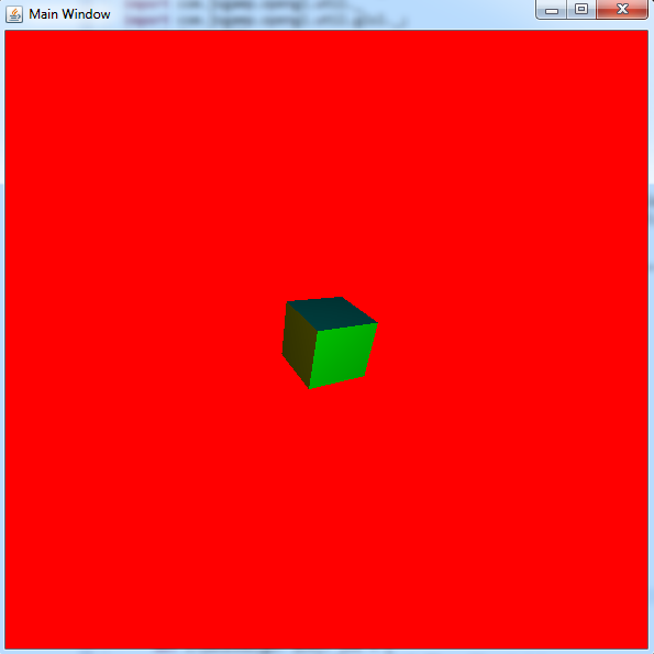
While the previous article on Scala and OpenGL was a bit lightweight, this one will serve to introduce many advanced concepts for basic 3D graphics. Our goal will be to render a basic, multicolored rotating cube like the one pictured below.

The first concept we need to understand is how our vertex data is fed into our vertex shader through the use of vertex buffer objects (VBOs) and vertex array objects (VAOs). To get started, let's create a float buffer containing all of our vertices. To do this I've constructed some basic utility objects and classes to make the process easier. First is a BufferUtil object that handles the logic of generating a VBO identifier, adding vertices to my float buffer and then storing in my VBO. object BufferUtils { def createBuffer(gl: GL4): Int = { val bufferArray: IntBuffer = IntBuffer.allocate(1); gl.glGenBuffers(1, bufferArray); return bufferArray.get(); } def createVAO(gl: GL4): Int = { val vaoArray: IntBuffer = IntBuffer.allocate(1); gl.glGenVertexArrays(1, vaoArray); return vaoArray.get(); } def setBufferData(gl: GL4, bufferID: Int, data: FloatBuffer): Unit = { //glBindBuffer sets the active array buffer to be manipulated. gl.glBindBuffer(GL.GL_ARRAY_BUFFER, bufferID); //Using GLBuffers utility class to provide the size of the float primitive so I can calculate the size val size: Long = data.limit() * GLBuffers.sizeOfGLType(GL.GL_FLOAT); gl.glBufferData(GL.GL_ARRAY_BUFFER, size, data, GL.GL_DYNAMIC_DRAW); } def addVertex(vertices: FloatBuffer)(x: Float, y: Float, z: Float): Unit = { vertices.put(x); vertices.put(y); vertices.put(z); vertices.put(1.0f); } }

The common theme you will begin to see is a reliance on the java.nio buffer objects and integer identifiers to identify the objects in the OpenGL API. The createBuffer() method above will allocate a new VBO identifier which we will need to keep track of through our program execution. It is needed because before we can perform work on the buffer we have to first bind it with a call to glBindBuffer(). After we have created our VBO and have a FloatBuffer of our vertices we can then store those vertices with a call to glBufferData() which will use the currently bound buffer to do its work.

But first we need to generate the vertices for our cube. bufferID = BufferUtils.createBuffer(gl); normalID = BufferUtils.createBuffer(gl); colorID = BufferUtils.createBuffer(gl); //2 triangles per face, 3 vertices per triangle, 4 elements per vertex, 6 faces = 144 vertices vertexCount = 144; val vertices: FloatBuffer = FloatBuffer.allocate(vertexCount); val normals: FloatBuffer = FloatBuffer.allocate(vertexCount); val colors: FloatBuffer = FloatBuffer.allocate(vertexCount); val addVertex = BufferUtils.addVertex(vertices)_; val addNormal = BufferUtils.addVertex(normals)_; val addColor = BufferUtils.addVertex(colors)_; vertices.clear(); normals.clear(); colors.clear(); addVertex(-0.5f, -0.5f, 0.5f); addVertex(0.5f, 0.5f, 0.5f); addVertex(-0.5f, 0.5f, 0.5f); addVertex(-0.5f, -0.5f, 0.5f); addVertex(0.5f, -0.5f, 0.5f); addVertex(0.5f, 0.5f, 0.5f); for(n <- 0 to 5) { addNormal(0.0f, 0.0f, 1.0f); addColor(1.0f, 1.0f, 0.0f); } addVertex(-0.5f, -0.5f, -0.5f); addVertex(-0.5f, 0.5f, -0.5f); addVertex(0.5f, 0.5f, -0.5f); addVertex(-0.5f, -0.5f, -0.5f); addVertex(0.5f, 0.5f, -0.5f); addVertex(0.5f, -0.5f, -0.5f); for(n <- 0 to 5) { addNormal(0.0f, 0.0f, -1.0f); addColor(0.0f, 1.0f, 0.0f); } addVertex(-0.5f, -0.5f, -0.5f); addVertex(-0.5f, 0.5f, 0.5f); addVertex(-0.5f, 0.5f, -0.5f); addVertex(-0.5f, -0.5f, -0.5f); addVertex(-0.5f, -0.5f, 0.5f); addVertex(-0.5f, 0.5f, 0.5f); for(n <- 0 to 5) { addNormal(-1.0f, 0.0f, 0.0f); addColor(0.0f, 0.0f, 1.0f); } addVertex(0.5f, -0.5f, -0.5f); addVertex(0.5f, 0.5f, -0.5f); addVertex(0.5f, 0.5f, 0.5f); addVertex(0.5f, -0.5f, -0.5f); addVertex(0.5f, 0.5f, 0.5f); addVertex(0.5f, -0.5f, 0.5f); for(n <- 0 to 5) { addNormal(1.0f, 0.0f, 0.0f); addColor(0.0f, 0.5f, 0.5f); } addVertex(-0.5f, -0.5f, -0.5f); addVertex(0.5f, -0.5f, -0.5f); addVertex(0.5f, -0.5f, 0.5f); addVertex(-0.5f, -0.5f, -0.5f); addVertex(0.5f, -0.5f, 0.5f); addVertex(-0.5f, -0.5f, 0.5f); for(n <- 0 to 5) { addNormal(0.0f, -1.0f, 0.0f); addColor(0.5f, 0.5f, 0.0f); } addVertex(-0.5f, 0.5f, -0.5f); addVertex(0.5f, 0.5f, 0.5f); addVertex(0.5f, 0.5f, -0.5f); addVertex(-0.5f, 0.5f, -0.5f); addVertex(-0.5f, 0.5f, 0.5f); addVertex(0.5f, 0.5f, 0.5f); for(n <- 0 to 5) { addNormal(0.0f, 1.0f, 0.0f); addColor(0.5f, 0.0f, 0.5f); } vertices.flip(); normals.flip(); colors.flip();

You will notice we are actually creating three buffers for our cube. In addition to the vertices for each cube face we are also specifying the normal vector and color of each vertex. In total there are 144 vertices that make up our cube since we have 6 faces with two triangles to form each face and three vertices to make a triangle. It is possible to reduce the number of vertices needed by changing the arguments passed to glDrawArrays() but for now we can keep things simple.

The normal and color data are necessary to compute the lighting and determine final color of each vertex in order to give the image some depth. The normal represents the direction each cube side is facing, therefore it is the same for all 6 vertices that make up that face. We also use the same color for all 6 vertices to make each face have its own color. I will discuss how these vectors are used when it comes time to write our shader.

Another thing worth mentioning is that all of our vertices are centered around the origin. These are technically already in what is called 'normalized device space' which is the region defined by the -1 to 1 range on all three axis. Anything that falls within this region will ultimately get transformed into window coordinates and displayed to the user. Normalized device coordinates are not particularly important at this point but centering the cube around the origin and making its dimensions 1x1x1 will also make the process of transforming it in the future much easier as well.

You may not realize it but there is actually some importance to the order that the vertices are arranged in order to get our cube to render properly. By default OpenGL will always render every triangle we specify. This does not work for us since we don't want to render the back side of the cube. To prevent this from happening we enable a feature called 'culling' which will only render triangles whos vertices are specified in a certain order. gl.glEnable(GL.GL_CULL_FACE);

By default trangles whos vertices are specified in counter-clockwise order are considered front-facing triangles and will be rendered to the user. This means when we construct the different faces of the cube we must take extra care use different vertex ordering for opposite faces since whenever one face is visible the opposite should not be visible.

Now that we have our buffers populated we make sure to call flip() and begin the process of feeding them into our VBOs and constructing our VAOs. BufferUtils.setBufferData(gl, bufferID, vertices); //Now that the vertex buffer object (VBO) is constructed we need to create a vertex array object (VAO) //The difference between the two is the VAO contains additional meta-data that describes //the formatting of the contents of the VBO. vaoID = BufferUtils.createVAO(gl); gl.glBindVertexArray(vaoID); //Attribute index 0 will obtain its data from whatever buffer is currently bound to GL_ARRAY_BUFFER and read it according //to the following specifications. gl.glVertexAttribPointer(0, 4, GL.GL_FLOAT, false, 0, 0); gl.glEnableVertexAttribArray(0); //setBufferData has the side-effect of changing the bound VBO BufferUtils.setBufferData(gl, normalID, normals); gl.glVertexAttribPointer(1, 4, GL.GL_FLOAT, false, 0, 0); gl.glEnableVertexAttribArray(1); BufferUtils.setBufferData(gl, colorID, colors); gl.glVertexAttribPointer(2, 4, GL.GL_FLOAT, false, 0, 0); gl.glEnableVertexAttribArray(2);

A VAO is essentially your VBO wrapped with additional data that describes the contents of the buffer. This data is provided through the call to glVertexAttribPointer() which will describe the currently bound VBO and store the information in the currently bound VAO. We create a single VAO to store all three of our buffers, making sure to allocate a unique index for each as the first parameter to glVertexAttribPointer(), those indices will ultimately be used for how we reference our data in the vertex shader. In the case of this application we describe our VBO as containing "4 component vertices of type 'float' that should not be normalized and is tightly packed (no data between vertices)".

At this point we are almost ready to render the cube, in fact, since it is already in normalized device space you could most likely make the call to glDrawArrays() and have the cube render properly. Although without any transformations you will be looking directly at one side of the cube and it will render as a plain square. To achieve the 3D affect we need to prepare some of our transformation vertices first. mvp.glMatrixMode(GLMatrixFunc.GL_MODELVIEW); mvp.glLoadIdentity(); val time: Long = System.currentTimeMillis(); val degrees: Float = ((time / 10) % 360); mvp.glTranslatef(0.0f, 0.0f, -5.0f); mvp.glRotatef(degrees, 1.0f, 1.0f, 0.0f); mvp.update(); //Modelview matrix gl.glUniformMatrix4fv(3, 1, false, mvp.glGetMatrixf()); //Normal matrix (transpose of the inverse modelview matrix) gl.glUniformMatrix4fv(4, 1, false, mvp.glGetMvitMatrixf()); mvp.glMatrixMode(GLMatrixFunc.GL_PROJECTION); mvp.glLoadIdentity(); //90 degree field of view, aspect ratio of 1.0 (since window width = height), zNear 1.0f, zFar 20.0f mvp.gluPerspective(90.0f, 1.0f, 1.0f, 20.0f); mvp.update(); //Projection matrix gl.glUniformMatrix4fv(5, 1, false, mvp.glGetMatrixf());

To make life easier I have used to JOGL PMVMatrix utility class to manage my matrices. This class has many valuable matrix operations for constructing, multiplying, storing and fetching matrix data used for your application.

The two matrices I work with in my application are the ModelView matrix and the Projection matrix. The ModelView matrix is what is responsible for moving my cube around and rotating it in place while the Projection matrix is what is responsible for translating my cube back into normalized device coordinates while also preserving the illusion that it is far off in the distance.

To construct my ModelView matrix I first change my matrix mode to ensure I am working on the right matrix and re-initialize it with the identity matrix (Matrix1 multiplied by the identity matrix = Matrix1). To achieve a constant spin I use the current system time and divide it by 10 to slow down the spin a little bit, then perform a modulus division to achieve a rotation degrees between 0 and 360. To perform my transformations I first multiply the identity matrix by a translation down the Z axis (into the screen) and then I multiply the resulting matrix by my rotation of x degrees on the X and Y axis. If you think about the order of operations however you may realize that this is backwards. In order to achieve an object spinning in place you should rotate then translate, otherwise the object will spin a wide circle around the axis of rotation. This strange ordering is explained in chapter 4 of the OpenGL SuperBible under the section labeled "Concatenating Transformations". It explains that is important to read transformations in reverse order. This behavior is closely tied to the order of how we perform our vertex transformations in the vertex shader which is usually a matrix multiplied by a vector.

To construct the Projection matrix I use the gluPerspective() method to construct a perspective projection. Another type of projection is the 'orthographic' projection but that typically used for 2D rendering, the perspective projection is what gives us the 3D appearance to simulate how things would appear in real life. The perspective projection is constructed by defining a 3D space bounded by field-of-view, screen ratio, near and far planes. In my case I went with a 90 degree field of view on the y-axis, an aspect ratio of 1 (this is normally viewport width divided by viewport height, in my case they are equivalent), a near plane located 1 unit down the z-axis and a far plane located 20 units down the z-axis. Any objects that are located within 3D space defined by these attributes will be transformed into normalized device space and rendered to the user. In order to render my cube I must move it down the z-axis by a few units in order for it to fall between the near and far planes ('down' referring to the negative z-axis which is the axis extending into the screen).

There is also usually a look-at matrix involved which is an additional transformation to simulate the effect of a movable camera. For this application you can just assume that our 'camera' is located at the origin staring down the negative z-axis.

Once our matrices are constructed we can feed them into our shader with calls to glUniformMatrix4fv(). Like our VAOs the first argument is a unique index that will be used to reference our uniform data in the vertex shader. It is referred to a 'uniform' because it is a single value that is constant amongst all of our vertices. This is different from data like normals and colors which could be unique for each vertex. You will also probably notice I snuck in an additional call to glUniformMatrix4fv after we configure the ModelView matrix. That call is responsible for providing the normal matrix we will use to transform our normal vectors. In most cases the normal matrix can be obtained by computing the transposed inverse of the ModelView matrix (which our PMVMatrix class gives us an easy method to obtain that value).

With all of our data prepared we can now construct our vertex shader #version 430 core layout (location = 0) in vec4 position; layout (location = 1) in vec4 normal; layout (location = 2) in vec4 color; layout (location = 3) uniform mat4 mvMatrix; layout (location = 4) uniform mat4 normalMatrix; layout (location = 5) uniform mat4 pMatrix; out vec4 intensity; void main(void) { gl_Position = pMatrix * mvMatrix * position; //Need to transform our normal to match the transformation of the position //This is done with the normal matrix which is the transposed inverse of the modelview matrix vec3 vNormal = normalize(vec3(normalMatrix * normal)); vec3 lightPos = vec3(0.0, 0.0, 1.0); vec3 vLight = normalize(lightPos - vec3(mvMatrix * position)); intensity = max(dot(vLight, vNormal), 0.0) * color; }

At the top you will see how we connect all of that data we just created to our shader inputs by using the location specifier when defining the input variables. Our shader will have two outputs, the built-in gl_Position vector and the intensity vector which contains the computed color after we perform our lighting calculations.

To obtain our modified position we first multiply our projection and modelview matrices together to obtain the pmvMatrix (projection-model-view matrix). We finally multiply this by our original position vertex to obtain the transformed vertex. If you remember our original vertex was inside normalized device space. This is true for our computed vertex as well except the computed vertex may have been moved to create the appearance of our cube being in the distance and rotating.

Lighting is a bit more difficult and can be abstract. To determine if the face of the cube should be illuminated we have to determine whether it is facing our light source or not. In this example I have put the light source at a fixed location on the positive z-axis (the axis extending towards you off the screen). If we take the position of the light source and the direction the vertex is facing (our normal vector) we can compute the angle between the two using the dot product equation. The dot product of two vectors is equal to the cosine of the angle between them times the lengh of the two vectors. If we normalize the vectors first (make their length equal to 1) then this equation simplifies and the dot product becomes equal to the cosine of the angle between the two vectors. If the two vectors are facing the same direction then the angle between them is 0 and the cosine of 0 is 1. This means the light source is hitting the vector directly and it should be completely illuminated. If the angle is between 90 degrees and 270 degrees then the vertex is facing off to the side or away from the light source and not be illuminated.

To start our lighting calculatation we multiply our normal vector by the normal matrix we created earlier and normalize the result since otherwise our normal vector would always be pointing at the original direction the cube face was pointed before we moved and rotated it. We also turn it into a 3 component vector since that last component is no longer important once we are done with our matrix transformations. To create the vector from our position to the light source we simply subtract the transformed position from the light position, making note to not include the projection transformation in this calculation since it is not related to where our vertex is located. Now that we have the vector from our vertex to the lightsource and the vector of where the vertex is facing we can compute our dot product. The resulting floating point value can then be multiplied against our original color to give it the appearance of becoming dark as it spins away from our light source. The computed intensity is passed out of our vertex shader where it will be used in our fragment shader to color our cube which is very simple: #version 430 core in vec4 intensity; out vec4 color; void main(void) { color = intensity; }

With our shaders ready to go we can finally make our call to glDrawArrays() and render the cube using the currently bound VAO. gl.glBindVertexArray(vaoID); //Draws the currently bound vertex array object gl.glDrawArrays(GL.GL_TRIANGLES, 0, vertexCount);

Additional Resources

Wolfram Alpha

Wolfram Alpha is a great website for working with mathematical calculations. It can be very valuable when you find yourself having difficulty visualizing the outcome of some of the vector operations performed by the shader.

OpenGL Wiki

The OpenGL wiki has some very useful articles explaining some of the behavior of OpenGL. This can be useful for filling in the gaps left behind by the API pages.

JOGL JavaDoc

Useful for understanding the differences between the JOGL API and their associated OpenGL API calls. There are also many valuable utility classes (like PMVMatrix) provided as part of the JOGL API.

It is generally undisputed that the best way to learn new languages is through applying them. Sometimes the difficulty with that approach is coming up with an idea that stresses your knowledge at a high level enough to solidify your skills. After all, the usual 'Hello World' program will only get you so far. My personal experience is that graphics and game development is something that can simultaneously spark your imagination and provide numerous opportunities to test your skills.

That said, I am neither an expert OpenGL developer nor am I an expert Scala developer. I have no technological justification for writing an OpenGL application in Scala, it is intended only as a learning exercise that may hopefully serve as a guidepost for others that which to do the same.

Since Scala is a JVM language we can thankfully rely on the existing libraries for OpenGL development in java. The one I have chosen to go with is JOGL in hopes that it more closely aligns with the core OpenGL API's in order to improve the chance that my knowledge transfers well to other languages like C++. There also exists a library called LWJGL that is designed more towards game development.

I will also be relying on the resources provided in the latest OpenGL Superbible for learning OpenGL. It can be difficult finding good information for learning OpenGL due to its long history. If you are not careful you may end up with a tutorial that teaches the old approach to OpenGL that relies heavily on the state machine versus the newer approaches that use vertex buffers and shaders.

Before any OpenGL application can start you will need to construct your application window. C++ applications usually rely on FreeGLUT to accomplish this. For Scala we can leverage the Swing/AWT API together with a GLCanvas object to construct the window we will render in. Here is the basic code snippit for doing this: object EntryPoint { def main(args: Array[String]): Unit = { val frameMain: Frame = new Frame("Main Window"); frameMain.setLayout(new BorderLayout()); val animator: Animator = new Animator(); frameMain.addWindowListener(new WindowAdapter() { override def windowClosing(e: WindowEvent) = { System.exit(0); } }); val canvas: GLCanvas = new GLCanvas(); animator.add(canvas); canvas.addGLEventListener(new Demo1()); frameMain.setSize(600, 600); frameMain.setLocation(200, 200); frameMain.add(canvas, BorderLayout.CENTER); frameMain.validate(); frameMain.setVisible(true); animator.start(); } }

We basically construct a simple frame and add a single canvas object to it. The animator is responsible for creating the typical application loop you see in OpenGL applications and the GLEventListener represents our main class with our render logic. The basic layout of a GLEventListener looks like this: class Demo1 extends GLEventListener { override def init(drawable: GLAutoDrawable): Unit = { } override def display(drawable: GLAutoDrawable): Unit = { } override def reshape(drawable: GLAutoDrawable, x: Int, y: Int, width: Int, height: Int): Unit = { } override def dispose(drawable: GLAutoDrawable): Unit = { } }

The init and dispose methods will be called at startup and shutdown of the animator loop. In our case the dispose method most likely doesn't get called when the application is closed since we do not make a call to 'animator.stop()' when the frame closes. In the init method we will initialize our shaders, program and vertex buffers. The display method will loop continuously in order to render each frame, this is where a lot of the application logic will ultimately be triggered from. The reshape method will be called whenever the window is resized, it is important for recalculating your perspective matrix but is not used in this project for now.

First things first, lets create the initialization logic for the application: object ShaderLoader { def createShader(gl: GL4, shaderType: Int, context: Class[_])(filename: String): ShaderCode = { ShaderCode.create(gl, shaderType, 1, context, Array(filename), false); } def createProgram(gl: GL4, shaders: ShaderCode*): ShaderProgram = { val retVal: ShaderProgram = new ShaderProgram(); retVal.init(gl); for(shader <- shaders) { retVal.add(shader); } return retVal; } } class Demo1 extends GLEventListener { override def init(drawable: GLAutoDrawable): Unit = { val gl: GL4 = drawable.getGL().getGL4(); val createVertexShader = ShaderLoader.createShader(gl, GL2ES2.GL_VERTEX_SHADER, this.getClass())_; val createFragmentShader = ShaderLoader.createShader(gl, GL2ES2.GL_FRAGMENT_SHADER, this.getClass())_; try { val vShader: ShaderCode = createVertexShader("shaders/vshader.glsl"); if(vShader.compile(gl, System.out) == false) throw new Exception("Failed to compile vertex shader"); val fShader: ShaderCode = createFragmentShader("shaders/fshader.glsl"); if(fShader.compile(gl, System.out) == false) throw new Exception("Failed to compile fragment shader"); program = ShaderLoader.createProgram(gl, vShader, fShader); if(program.link(gl, System.out) == false) throw new Exception("Failed to link program"); //No longer needed vShader.destroy(gl); fShader.destroy(gl); val vertexArrays: IntBuffer = IntBuffer.allocate(1); gl.glGenBuffers(1, vertexArrays); vBuffer = vertexArrays.get(); } catch { case e: Exception => { e.printStackTrace(); System.exit(1); } } } }

In this you can see that I have created a ShaderLoader object to help reduce some of the boilerplate with creating shaders and programs. By using currying and partial defined functions I am able to create two helper methods that simply take filenames of the shader source files I wish to load. JOGL also defines helper classes named ShaderCode and ShaderProgram for creating and managing your OpenGL objects, versus the normal way of managing a bunch of abstract integer values. The basic flow is to fist create your shaders and compile them, add them to a program and then link the program, the one piece of information you need to retain after doing all of this is the program identifier. That identifier will be used during the display loop together with vertex arrays/buffers in order to render objects.

The shaders used for this application are simple and were pulled from the first sample in the OpenGL Superbible. Our vertex shader takes no input and produces a hardcoded value as the output position: #version 430 core void main(void) { gl_Position = vec4(0.0, 0.0, 0.5, 1.0); }

Our fragment shader also takes no input and produces a hardcoded color value as the output: #version 430 core out vec4 color; void main(void) { color = vec4(0.0, 0.8, 1.0, 1.0); }

Normally the vertex shader would be provided a vertex as input which we could then manipulate with things like our MVP matrix to controls its position in our 3D world. For now we will basically render a point directly in the middle of the screen. The fragment shader would normally also be provided information on how to color each vertex, or perhaps information related to a texture, that would then be interpolated between vertices. Our fragment shader however will always set the color of each vertex to a hardcoded value.

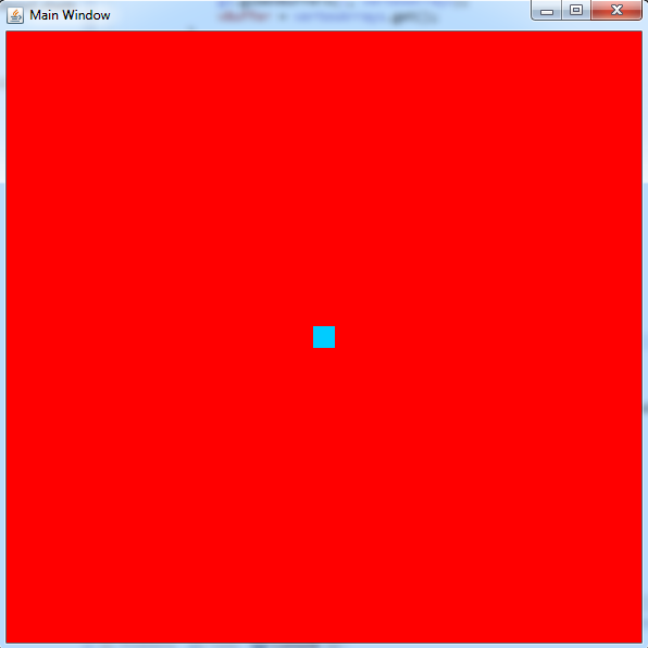
With our application initialized and our shaders created we can create our code to actually draw something: override def display(drawable: GLAutoDrawable): Unit = { val gl: GL4 = drawable.getGL().getGL4(); val redArray: Array[Float] = Array(1.0f, 0.0f, 0.0f, 1.0f); gl.glClearBufferfv(GL2ES3.GL_COLOR, 0, redArray, 0); program.useProgram(gl, true); gl.glBindVertexArray(vBuffer); gl.glPointSize(20.0f); gl.glDrawArrays(GL.GL_POINTS, 0, 1); }

This will set the default color of all pixels to red with a call to glClearBufferfv. After that we set the program we created during intialization to our active program, this means that any vertices rendered with glDrawArrays will be processed using the shaders linked to that program. The call to glBindVertexArray will specify which set of vertices will be fed into the shaders, this data is not actually used for the application but is still necessary. For now we are going to render a single point on the screen which is why we passed in 'GL.GL_POINTS', we also increase the size of that point with a call to glPointSize to make it easier to see. If we wanted to render triangles or other objects we would change the first argument to 'glDrawArrays' to something else, but that will also require additional vertices to work. For example you would need at least three vertices in order to render a triangle.

When we run the program this is what we see:

You can download the files for this project here: Download Project Files. They are compatible with the Scala SDK version 3.0.2 for Windows x86_64.

When writing an API there is often a trade-off that happens when you struggle with long argument lists. Sometimes you end up introducing more stateful information to an object and exchange horizonal verbosity for vertical verbosity. This is most frequently demonstrated with the use of the factory pattern to which introduces helper classes to help construct complex objects. Unfortunately some APIs take this to the extreme and you find yourself surrounded by factory objects, even in situations where they might not have been needed.

One feature of Scala that I have found interesting is the use of function currying and partially defined functions. This can provide a valuable third option for improving the usability of an API without having to resort to the factory pattern every time. Take for example the following function: def glBeginEnd(objType: Int)(beforeEnd: => Unit)(actions: (Int) => Unit): Unit = { gl.glBegin(objType); for(i <- 0 to teeth) { actions(i); } beforeEnd; gl.glEnd(); }

The above is a snippit from a Scala implementation of the popular OpenGL gears application. When given a number of teeth (captured via a closure) it will perform actions on each integer to construct the vertices for the individual tooth of the gear. For the most part however the first two arguments may not be used frequently and therefore become annoying noise in the invocation of the function. If I use function currying to separate those arguments I can create a partially defined function where those two arguments are already set: val createQuadStrip = glBeginEnd(GL2.GL_QUAD_STRIP)({ })_;

This will make future invocations of the function to something like: createQuadStrip((i: Int) => { //generate vertices for tooth 'i' });

And it will construct a quad strip graphic based off the vertices generated by my function parameter. I will admit that three parameters is hardly a long argument list for a method, but I do think it demonstrates a good application of this functionality. By grouping parameters based on how frequently they will change you can allow the user of the API to eliminate some of those parameters early on and produce a partially defined function that performs what they need in a more precise and readable manner.

You can view the full source of the Scala OpenGL gears application here.

In a strange coincidence I found myself in two issues related to symbol collisions the past few days. The difficult part about these kind of problems is they can manifest in the strangest ways. In both cases I ran the application through a debugger and witnessed as the value for a variable suddenly become invalid as it was passed from one function to another when there was nothing else that was acting on that variable. This resulted in a lot of unexplainable segmentation faults and other severe application malfunctions.

The first situation was triggered when I was trying to build some third-party libraries for our application. In some scenarios we prefer to add a prefix to the libraries to avoid situations where we would accidentally pick up a copy that might already be installed on the customer's machine. In order to properly rename a shared library you need to change the SONAME that is stored in the dynamic section (ELF Format), simply renaming the shared library file is not sufficient. In my attempts to modify the build process to generate the correct SONAME I somehow triggered it to include all of the symbols of Library A inside Library B as well. Once I recognized that the file sizes of the generated libraries did not look correct I inspected their symbol tables with `nm` and discovered that the method that was crashing was defined in both. After adjusting the build again I was able to get it to generate the libraries without duplicating the symbols.

The second situation was triggered when a co-worker copied a codebase to write a new component since he needed most of the same functionality with only minor modification. Unfortunately, when copying large chunks of code it is very easy to forget to change everything that needs to be changed. In this case he forgot to change the namespace and class names of some of the components which resulted in duplicate symbols. An innocent mistake that manifested with a segmentation fault only when both modules were in use. Once I identified the overlapping symbols by examining the `nm` output I was able to rename the namespaces in the new module to resolve the conflict.

Unfortunately most of our code base dates back before some useful mechanisms for avoiding symbol collisions came into play. For example, GCC 4.X introduced the flag "-fvisibility" to control the default symbol visibility. You can find more documentation on it's functionality and benefits here

When the number of machines in a production environment begin to surpass the double and triple digits the problem of managing them quickly rises to the top. When these machines are involved with sensitive information the problem snowballs into not only ensuring the performance and stability of the machines but also things like intrusion and vulnerability detection. Since it would take a small army of highly trained individuals to manually monitor these machines companies will often attempt to create solutions that would bring managing thousands of machines into the realm of possibilities.

Unfortunately there are still limitations with home-grown solutions. It is very difficult to keep up with all of the published regulations and known vulnerabilities on top of acquiring the skilled individuals to maintain such a solution. They have essentially traded one problem for another. This has created an industry of companies that attempt to provide solutions to those trying to tackle this problem.

Regardless of your chosen solution, the most difficult task faced is finding the information you need and getting it off the machine. There are usually two competing philosophies for obtaining this information, agents versus agent-less.

However, if you define an 'agent' as a process that sits on the machine and exposes information through a network interface then both types of solutions are essentially agent-based. The difference is that in an 'agent-less' solution the 'agent' is a common application that is either shipped with the OS or is easily obtained and installed. Versus a true agent based solution is one that provides a piece of proprietary software that must be installed on all the monitored systems.

This does not mean that agent-less has no advantages. Deploying and managing agents is very, very difficult in large environments. A solution that leverages a component that can be automatically found on every machine can produce a quick return for your investment at very little cost. On the downside, this means the solution is limited by the capabilities of whatever utility they commandeer to act as their agent. There may be features you want but will never be fulfilled because the creators of the solution have no control over their 'agent'. This also means that if the agent breaks or does not function properly you will have to go through another party for support.

An agent-based solution on the other hand provides more features in exchange for complexity and cost of ownership. The solution provider must commit to providing not only the agent but the tools to manage it as well. This makes it very costly for a solution provider to develop and maintain an agent because it is a piece of software that will be installed thousands of times across a wide variety of environments. There are many cases where the agent will not function properly because it is not robust enough to handle extreme environments (resource starved servers for example). Some of this stems from the additional complexity that is created as features are added to the agent. This provides value to the user of the product but creates more potential for problems. Your success with an agent-based solution will rely heavily on the quality of support that comes with the solution.

This doesn't mean that agent-less solutions are rock-solid but statistically speaking a piece of software that gets installed automatically with every OS has had more opportunities to identify problems and solve them.

The best solution depends on the problem you are trying to solve and the solution being presented. An agent-based solution that lacks the infrastructure to maintain and support the agent is just as useless as an agent-less solution that is unable to provide the features you need to accomplish your goals. Companies like to gravitate towards producing agent-less solutions because that also means less development and maintenance costs (they are basically offloading the work to a third party). It is important to identify the limitations of agent-less solutions and consider the chance that you will outgrow the solution. When presented with an agent-based solution you should consider the cost of deploying and maintaining the agents on your hardware and ask the company what tools are provided to mitigate that cost while not letting it distract you with all the features it promises.

Sqlplus is a command line utility that is provided with the Oracle database which allows you to connect to the database and perform commands or queries against it. One way to use it is to log in as the oracle user account and execute the following shell commands (assuming this is a Linux/Unix based install of the Oracle database). export ORACLE_SID=orcl export ORACLE_HOME=/home/oracle/app/oracle/product/11.2.0/dbhome_1 export PATH=$ORACLE_HOME/bin:$PATH

In the above example I obtained the ORACLE_SID and ORACLE_HOME values from my /etc/oratab file. With my environment prepared I can now execute the sqlplus command. sqlplus / as sysdba

This will start up a sqlplus session and connect to the database using the credentials of the Unix user I am running as (which should be the 'oracle' user) with DBA privileges. If you wanted to use a restricted user account you could do something like: sqlplus username/password

Or you can even start an unconnected session and manually use the 'connect' command: sqlplus /nolog SQL>connect username/password

This all works fine running sqlplus as the 'oracle' user. But what happens when we break that assumption? Well you might see this error: ERROR: ORA-12546: TNS:permission denied

Or in more severe cases you may discover that the sqlplus command hangs and never returns.

What actually happens when the sqlplus utility attempts to connect to the database is it will fork and exec a child process using the 'oracle' binary: execcve("/u01/app/oracle/product/11.2.0/db_1/bin/oracle", ["oracleorcl", ...) = 0

The ORA-12546 error usually stems from the fact that the user you are running as lacks permission to access that binary. This is probably because one of the parent folders does not have read and execute permission for 'others'. However if you attempt to fix the problem by changing the permissions on that folder you will run into the second problem I mentioned where the sqlplus command hangs.

What happens in that case is the exec call is successful and the oracle binary starts execution and then early into its execution it gets stuck in an endless loop of attempting to find an audit log file to write to: access("/u01/app/oracle/admin/orcl/adump/orcl_ora_20498_1.xml, F_OK) = -1 EACCES (Permission denied) access("/u01/app/oracle/admin/orcl/adump/orcl_ora_20498_2.xml, F_OK) = -1 EACCES (Permission denied) access("/u01/app/oracle/admin/orcl/adump/orcl_ora_20498_3.xml, F_OK) = -1 EACCES (Permission denied) access("/u01/app/oracle/admin/orcl/adump/orcl_ora_20498_4.xml, F_OK) = -1 EACCES (Permission denied) ...

The EACCES return code tells us that there is still some sort of permission issue here. This may seem strange if you started sqlplus as the root user. What is even more strange is if we examine the 'oracle' binary that is passed to the exec call we will see that it has it's setuid and setgid bits set -rwsr-s--x 1 oracle oinstall 173515477 Sep 8 2011 oracle

This means that execution of this binary will have the side effect of changing the effective user and group ids to 'oracle' and 'oinstall' which should also have access to create an audit log file in the 'adump' directory. So why is it failing still?

There are actually two things happening here that are not immediately obvious. If we examine the strace output of an sqlplus session running as a non-oracle user we see that a check to 'geteuid' is called followed shortly by a call to 'setuid(2)' after we fork but before we exec the oracle binary. This means that the real UID of the oracle binary becomes 2 (usually the 'daemon' user on Linux machines). So what right? We will still be changing it to 'oracle' when the oracle binary executes. Not quite. If you read the man page for the 'access' command you will see: The check is done using the calling processes real UID and GID, rather than the effective IDs as is done when usually attempting an operation on the file.

This means that our 'access' call is done using the permissions of the 'daemon' user and will fail as a result.

To fix this problem you can add the user you want to run sqlplus as to the 'oinstall' group. Since there is no call to 'setgid' or 'initgroups' by the sqlplus command this permission will cascade all the way through and the oracle binary will have 'oinstall' as both the effective and real group permission which should allow the 'access' call to pass.

Scala is an interesting and powerful language I picked up a while back and although I have not had many chances to incorporate it into my daily work it has been a valuable learning tool. The fact that it is a language that runs on the JVM makes it possible to continue using many of the same APIs and libraries that makes Java such a powerful language.

And with the direction many popular languages are evolving it is becoming more important to familiarize yourself with functional programming. For example, Java 8 should hopefully introduce support for lambda expressions into the language which is something Scala developers are very familiar with.

If you have done some Swing development you might be familiar with this pattern: SwingUtilities.invokeLater(new Runnable() { override def run(): Unit = { //Update UI }});

With a little bit of Scala magic we can eliminate a lot of the boilerplate to make life easier. object SimpleUtilities { def invokeLater(action: => Unit): Unit = { SwingUtilities.invokeLater(new Runnable() { override def run(): Unit = { action; }}); } }

Which turns the original call into this: SimpleUtilities.invokeLater { //Update UI }

By taking advantage of a parameterless lambda function argument we are able to create something that is much cleaner and almost feels like we are altering the languages' syntax.

I was recently tasked with understanding how to reconfigure a machine's syslog daemon to route its traffic to a non-standard port. If you find yourself using a modern variant of syslog such as rsyslog (common on many versions of Linux) this is often a simple task of adding the port to the end of the syslog target: *.debug @@targethost:targetport

But if you are working on old machines or variants of UNIX that have not moved away from the classic syslog daemon it is often unclear how to configure this behavior. In fact if you were to attempt the same line above the entire string after the '@' symbol will be taken as the hostname and it will be considered an unroutable destination.

Surely the answer is as simple as reading the manual page or a google search but surprisingly enough it is not a common task people need to perform. It was only after reading stories from customers attempting to do the same thing was I reminded of the purpose of the '/etc/services' file you will find on most UNIX machines.

This file contains a list of registered ports and their services that the system can use as a reference for various purposes. For example, when performing a `netstat` command it will automatically translate the port number into a human readable service name to help improve understanding of the output. Proto Recv-Q Send-Q Local Address Foreign Address State tcp 0 0 *:http *:* LISTEN tcp 0 0 *:ssh *:* LISTEN

If you wanted to view the port numbers you can override this behavior with the '-n' option for `netstat`. Proto Recv-Q Send-Q Local Address Foreign Address State tcp 0 0 0.0.0.0:80 0.0.0.0:* LISTEN tcp 0 0 0.0.0.0:22 0.0.0.0:* LISTEN

It turns out that by editing the port that syslog is registered under in this file you can control what port the syslog daemon uses to send data to. So by simply flipping one line in /etc/services from syslog 514/udp

to syslog 1514/udp

and restarting the syslog daemon you are able to change the port being used.

Things started to get really tricky when I was alerted that even with the above steps it was still not possible to change the syslog behavior on AIX platforms. Once again I was unable to find the information I needed in the usual documentation. There must be some way of investigating what configuration files the syslog daemon uses to configure itself, other than the obvious '/etc/syslog.conf'.

Now if I had the source code I could probably just examine the syslog implementation to understand what additional config files I should look at, but unfortunately it is not always easy to get the right copy of the source. Instead I had to turn to a useful low-level tool I use for investigating basic application system calls.

On AIX the name of this tool is `truss` (alternatively named `strace` on other platforms) and it shares a lot of behavior in common with `gdb`. It will allow you to attach to a running process or launch an application under it and view the low level system calls (file opens, libraries being loaded, etc).

Using this tool I am able to capture all of the configuration files that are being loaded by the syslog daemon when it starts. The syntax for this is: truss -f syslogd > truss.out 2>&1

Which will run the syslogd binary under the truss command, following any children created by fork calls and redirecting all the output to a file so I can easily view it.

In that output I am able to examine each file open and view the man page for anything that looks like a configuration file. This eventually let me to a file on AIX called '/etc/irs.conf'. The purpose of this file is to instruct the machine on what order it should use to resolve various bits of information. For example, if you wanted to resolve a hostname from your '/etc/hosts' file before attempting to resolve it through DNS you could add a line to this file like so: hosts local dns

In my case, what I wanted to do was add a single line services local

Which would instruct my machine to honor the information in the local '/etc/services' file that contained my altered syslog port. With this change in place I was able successfully get my syslog daemon to start sending data to the correct port.

Working with multi-threaded applications can be difficult at times until you can reconcile your threading model. You may find yourself in situations where the application encounters a deadlock and you need to figure out what threads are competing for control.

If you are debugging a C/C++ application you may end up using the GDB debugger to examine the application call stack. Using GDB can be a bit intimidating for those that have not used it before but with knowledge of a few critical commands it can be a very valuable tool.

So lets say your application is locked up and you have managed to connect GDB to it. Your first step is to probably grab a list of the threads. (gdb) info threads

For which you might see something like: Id Target Id Frame 29 Thread 0x7f7f99b18700 (LWP 16597) "chromium-browse" 0x00007f7f9ed5b88d in waitpid () 28 Thread 0x7f7f93586700 (LWP 16598) "NetworkChangeNo" 0x00007f7f9cc77619 in syscall () 27 Thread 0x7f7f92d85700 (LWP 16599) "inotify_reader" 0x00007f7f9cc74763 in select () 26 Thread 0x7f7f92584700 (LWP 16602) "AudioThread" 0x00007f7f9ed57d84 in pthread_cond_wait@@GLIBC_2.3.2 () 25 Thread 0x7f7f90946700 (LWP 16603) "threaded-ml" 0x00007f7f9cc6fa43 in poll () 24 Thread 0x7f7f77ffe700 (LWP 16604) "CrShutdownDetec" 0x00007f7f9ed5ad2d in read () 23 Thread 0x7f7f775f5700 (LWP 16605) "Chrome_DBThread" 0x00007f7f9ed57d84 in pthread_cond_wait@@GLIBC_2.3.2 () 22 Thread 0x7f7f76df4700 (LWP 16606) "Chrome_FileThre" 0x00007f7f9cc77619 in syscall () 21 Thread 0x7f7f765f3700 (LWP 16607) "Chrome_FileUser" 0x00007f7f9ed57d84 in pthread_cond_wait@@GLIBC_2.3.2 () 20 Thread 0x7f7f75df2700 (LWP 16608) "Chrome_ProcessL" 0x00007f7f9ed57d84 in pthread_cond_wait@@GLIBC_2.3.2 () 19 Thread 0x7f7f755f1700 (LWP 16609) "Chrome_CacheThr" 0x00007f7f9cc77619 in syscall () 18 Thread 0x7f7f74df0700 (LWP 16610) "Chrome_IOThread" 0x00007f7f9cc77619 in syscall () 17 Thread 0x7f7f57fff700 (LWP 16611) "IndexedDB" 0x00007f7f9ed57d84 in pthread_cond_wait@@GLIBC_2.3.2 () 16 Thread 0x7f7f572ec700 (LWP 16612) "BrowserWatchdog" 0x00007f7f9ed57d84 in pthread_cond_wait@@GLIBC_2.3.2 () 15 Thread 0x7f7f56aeb700 (LWP 16614) "BrowserBlocking" 0x00007f7f9ed57d84 in pthread_cond_wait@@GLIBC_2.3.2 () 14 Thread 0x7f7f562ea700 (LWP 16615) "BrowserBlocking" 0x00007f7f9ed57d84 in pthread_cond_wait@@GLIBC_2.3.2 () 13 Thread 0x7f7f54ae5700 (LWP 16617) "Proxy resolver" 0x00007f7f9ed57d84 in pthread_cond_wait@@GLIBC_2.3.2 () 12 Thread 0x7f7f349ef700 (LWP 16618) "MediaStreamDevi" 0x00007f7f9ed57d84 in pthread_cond_wait@@GLIBC_2.3.2 () 11 Thread 0x7f7f2ecdb700 (LWP 16619) "Proxy resolver" 0x00007f7f9ed57d84 in pthread_cond_wait@@GLIBC_2.3.2 () 10 Thread 0x7f7f2e4da700 (LWP 16620) "Chrome_SafeBrow" 0x00007f7f9ed57d84 in pthread_cond_wait@@GLIBC_2.3.2 () 9 Thread 0x7f7f2cecb700 (LWP 16621) "renderer_crash_" 0x00007f7f9ed57d84 in pthread_cond_wait@@GLIBC_2.3.2 () 8 Thread 0x7f7f1b7fe700 (LWP 16626) "Chrome_HistoryT" 0x00007f7f9ed580fe in pthread_cond_timedwait@@GLIBC_2.3.2 () 7 Thread 0x7f7f1bfff700 (LWP 16629) "extension_crash" 0x00007f7f9ed57d84 in pthread_cond_wait@@GLIBC_2.3.2 () 6 Thread 0x7f7f1a7fc700 (LWP 16636) "NSS SSL ThreadW" 0x00007f7f9ed57d84 in pthread_cond_wait@@GLIBC_2.3.2 () 5 Thread 0x7f7f1affd700 (LWP 16639) "CachePoolWorker" 0x00007f7f9ed57d84 in pthread_cond_wait@@GLIBC_2.3.2 () 4 Thread 0x7f7f1925b700 (LWP 16647) "CachePoolWorker" 0x00007f7f9ed57d84 in pthread_cond_wait@@GLIBC_2.3.2 () 3 Thread 0x7f7f18a5a700 (LWP 16653) "BrowserBlocking" 0x00007f7f9ed57d84 in pthread_cond_wait@@GLIBC_2.3.2 () 2 Thread 0x7f7f55ae9700 (LWP 16682) "CachePoolWorker" 0x00007f7f9ed57d84 in pthread_cond_wait@@GLIBC_2.3.2 () * 1 Thread 0x7f7f99dec980 (LWP 16585) "chromium-browse" 0x00007f7f9cc6fa43 in poll ()

You can use the backtrace command to get a detailed stack trace of the currently selected thread (denoted by the * next to it). (gdb) bt #0 0x00007f7f9ed57d84 in pthread_cond_wait@@GLIBC_2.3.2 () from /lib/x86_64-linux-gnu/libpthread.so.0 #1 0x00007f7faa1c6527 in base::SequencedWorkerPool::Inner::ThreadLoop(base::SequencedWorkerPool::Worker*) () from /usr/lib/chromium-browser/libs/libbase.so #2 0x00007f7faa1c6c0b in base::SequencedWorkerPool::Worker::Run() () from /usr/lib/chromium-browser/libs/libbase.so #3 0x00007f7faa1c6eb9 in base::SimpleThread::ThreadMain() () from /usr/lib/chromium-browser/libs/libbase.so #4 0x00007f7faa1c32c4 in ?? () from /usr/lib/chromium-browser/libs/libbase.so #5 0x00007f7f9ed53e9a in start_thread () from /lib/x86_64-linux-gnu/libpthread.so.0 #6 0x00007f7f9cc7b3fd in clone () from /lib/x86_64-linux-gnu/libc.so.6 #7 0x0000000000000000 in ?? ()

To view information on other threads you can switch between them. (gdb) thread 2 [Switching to thread 2 (Thread 0x7f7f55ae9700 (LWP 16682))] #0 0x00007f7f9ed57d84 in pthread_cond_wait@@GLIBC_2.3.2 () from /lib/x86_64-linux-gnu/libpthread.so.0

But switching each thread to view the backtrace can be a bit tedious. So here's a useful way to view all of them at once: (gdb) thread apply all bt

Those familiar with bash shells can even take this one step further. gdb > threads.txt 2>&1 <<END attach $PID thread apply all bt quit END

The above snippit automates the process of connecting to your running application (replace $PID with the actual process ID) and recording the backtraces of all of the threads to a file. This will allow you to investigate the threading information more easily in a text editor you are comfortable with.

Hopefully at this point you have managed to gather the information you need to understand what your threads are deadlocking on.

I was recently working on creating a sychronized interface to an asynchronous communication library and while performing stress tests against it I discovered some interesting threading behavior that may be worth mentioning. Basically the design of the asynchronous library involves two threads, the calling thread and the responding thread. The calling thread initiates the request and returns immediately without waiting for a response. Eventually the remote server will respond to the request and the responding thread will dispatch the response. The responding thread is usually always running and monitoring the connection to the remote server, while there may be multiple calling threads phasing in and out of existence to generate requests.

My task was to create a version of the API that would block until the response was returned, thus making it behave like most communication API's you would normally be used to.

To do this I introduced a synchronizer object that would then be passed between the two threads through a user data object. The calling thread would initialize the synchronizer, make the request, and then lock on it. The responding thread would then obtain the same synchronizer reference through the user data object and when the response came back it would populate the synchronizer with the results of the call and unlock it. When the lock call returns in the calling thread we can then access the results of the response that were stored in the synchronizer.

There are some obvious things you have to worry about with this implementation. For example, the response may arrive before the calling thread can execute the lock method on the synchronizer.

And then there are some more nefarious issues that may not be immediately obvious. In this case, since the responding thread was always running it may not always see the same picture as the calling thread. If, for example, the calling thread creates a new object at the time you make a request, the responding thread may not see the same copy of that object. It may simply see a partially instantiated version of this object, especially if it is a complex data type. This is because the fully instantiated copy of the object may only be in the calling thread's CPU cache and has not been persisted to memory or the responding thread's CPU cache (granted this is probably a very naive explanation for what is actually happening).

You can fight this issue through the use of a memory barrier that will flush out the store/load buffers and ensure both CPUs have the same copy of the object in their cache. In my case, a simple pthread_mutex should suffice as an appropriate memory barrier. The basic rule here is if both threads lock on the same mutex then thread B is guaranteed to at least see the same state of memory from the moment thread A released the same mutex. This behavior is usually accomplished by enforcing rules on the order of the load and store operations performed by the threads.

Except one problem...

The mutex was my complex data structure that was being corrupted. This was because the mutex I was trying to use was being instantiated as part of my synchronizer object that was created at the moment the calling thread made a request. To create a proper memory barrier I needed at least one mutex that was created before the responding thread ever started, which may have been much further back in the applications execution.

After passing this hurdle I continued my tests on the implementation and eventually tripped on an even stranger version of this behavior. My calling thread was instantiating an object, passing it to the responding thread as part of the request, and then would crash when the method finished executing and attempted to deconstruct the object. So if the calling thread created the object and I can observe that the responding thread does not interact with it as part of the request, then how can that same data structure be corrupt when the same thread that created it tries to deconstruct it?

What I discovered was a variation on the previous issue. In this case the responding thread had an incomplete representation of the object in its cache and then it initiated the memory barrier first, making its copy the authoritative copy. This in turn updated the copy in the calling thread which then caused issues when we tried to deconstruct an incomplete object. The solution to the problem was to make sure that any data object that was created at the time of the request was guarded first by the mutex that was being used for the memory barrier. This guaranteed that version of the object in the calling thread's cache became the authoritative copy.

What is interesting is this topic as a whole is not commonly talked about, which can make it hard to research and understand what is actually happening here. Usually when you discuss threading issues you will commonly talk about race conditions and deadlocks. Part of the reason this issue does not get attention is it is often dependent on the architecture you are developing against. I first learned about this in Java Concurrency in Practice where similar behavior can be observed due to the memory model used by the java virtual machine. In the problem described above I was actually developing a C++ application on an x86 Linux platform. Some useful documentation describing the use of memory barriers on Linux can be found here

We had a reasonably simple race condition in the code that created a situation where one thread could generate a report based off data stored in two queues at the moment both queues were empty because the data was being transitioned between them.

Check in the code change, test it, generate a patch for the product, ship the patch to the customers.

Problem solved.

Until a few weeks later when users started reporting that the issue was still reproducing.

In response we scoured the source code. Surely there was some other threading issue hiding from us. Was there some other location this data was being accessed or the queues were being manipulated that was not properly guarded by our locking mechanism?

A week of work, endless hours of speculating and testing the most bizarre kinds of threading issues and nothing indicated why the problem would still exist. Until someone asked the most obvious of questions "Are we sure it was included in the patch?".

This triggered a completely new line of investigation into our build process where we were finally able to put the pieces together. The original fix for the problem was to code that was stored in a header file. Since our build was incremental and lacked a 'makedepend' step this means there is a manual step to force a build of the object file by touching a .cpp file. In this case, since the code was in a header file the appropriate .cpp file that needed to be touched was not the associated .cpp file but the .cpp file that included the call to that function. This meant that the wrong object file was compiled and shipped to the user and they never obtained the original fix.

The takeway from this was: use makedepend, avoid code in header files, start every problem by challenging your basic assumptions.

FIPS 140-2 is a cryptographic regulation used commonly by government agencies. There are pages of documentation describing the regulation in detail but for software applications it can be best summarized into two important rules:

1. Only use algorithms from the approved list (ciphers, hashes, key negotiation, etc).
2. Steps must be taken to preserve the integrity of the cryptographic module

The first requirement is usually not that difficult to achieve. Just turn off the algorithms not included on the list and you are good to go.

FIPS becomes complicated when trying to meet the second requirement. There are actually four defined security levels for FIPS and if you are using a software module (such as OpenSSL or Mozilla's NSS) then only levels 1 and 2 apply to you. This is because level's 3 and 4 begin to talk about requirements such as tamper proof casing that can only be applied to hardware modules.

In the case of OpenSSL the second requirement is accomplished through a very specific build process that embeds a precomputed hash of the module. This hash is then compared against the in-memory representation of the module when your application starts and initiates FIPS mode of operation.

The build for OpenSSL is so precise that if you do not follow the handful of commands outlined in their FIPS user guide then you will break compliance. In fact, even basic steps such as how you obtain the packages for building your OpenSSL distribution have to be done properly to ensure you retain compliance.

And just because you have managed to build it does not mean you are out of the woods. On newer versions of Windows you may discover that the self-test fails to properly confirm the integrity of the module. This is because the module expects to load at a preferred base address and if that address is not available then it will cause the self-test to fail. The best advice to resolve these issues are to toy with alternate base addresses and ensure that the module is loaded at the earliest possible moment during application execution. In my case I was loading the module to be used by JNI calls made by the JVM. The overhead of the JVM and the late loading time of the module practically ensured that it would load too late and the base address would not be available. I was able to resolve the issue by changing the linking behavior of my JNI libraries to ensure that the OpenSSL library was loaded as a dependency during program startup rather than later as a call to LoadLibrary.

All this aside, is FIPS truely safer?

Are the algorithms more secure? That's hard to say. Sure, disabling the weaker algorithms is a good thing but under normal operation your application was likely to negotiate to use the strongest algorithm available. In fact, due to the slow turnaround time in creating FIPS approved modules (this involves a long, expensive, certification process), we create situations where newer and more secure algorithms are not included because they have not yet made their way into the FIPS standard.

Then it must be more secure because of the integrity checks, right? But how can you be sure that the module I provided you was built the correct way? Maybe I just slapped a big "FIPS Inside" sticker on the product box and put it on the shelf?

Unfortunately it is very difficult for the consumer to confirm where or not my application is using FIPS properly. I could have just as easily added a single line of code that printed out the message Enabling FIPS....Success!

Rather than calling the correct methods for triggering the FIPS integrity checks.

Perhaps what we really need is a central authority providing prebuilt and certified modules that could then be dropped into the application by the user, rather than shipped with the application. That way the user can at least verify that the copy they have matches what was published by the authority and removes the chances of mistakes made by the application provider when building their own copies of the modules.